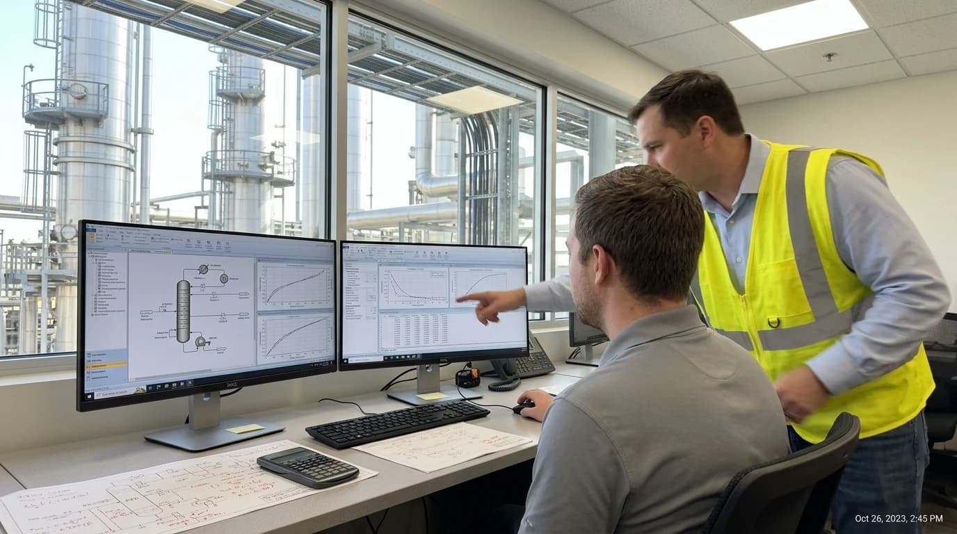
Multi-Component Distillation Simulation: NRTL vs PR
Resolving column convergence to cut distillation energy consumption by up to 15%.
Multi-component distillation simulation is a computer-based modelling technique used by process engineers to calculate the phase equilibrium, heat duties, and mass transfer rates within fractionation columns separating mixtures of three or more chemical species. In modern industrial operations, distillation represents the primary method of separation, yet its operational costs are high. Industrial separation processes consume roughly 10% to 15% of total industrial energy, with distillation alone accounting for approximately 3% of global energy consumption. In typical petrochemical refineries and speciality chemical production facilities, distillation units manage over 40% of all separation duties, rendering column optimisation a priority for industrial decarbonisation.

Heat & Mass Balance.
Map every energy and material flow in your process with detailed heat and mass balance calculations — the foundation for any optimisation or design project.
Fundamentals of Multi-Component Distillation Simulation
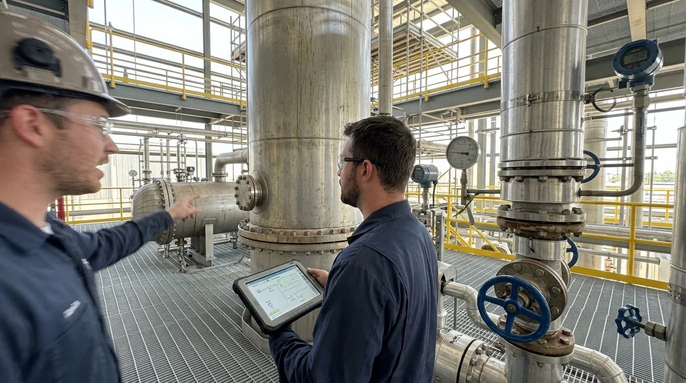
Industrial operators face intense regulatory pressure to lower their scope 1 and scope 2 greenhouse gas emissions. In the United Kingdom, facilities must comply with the environmental thresholds outlined in the Environmental Permitting (England and Wales) Regulations 2016. In the European Union, the Industrial Emissions Directive 2010/75/EU enforces Best Available Techniques (BAT) to limit energy consumption and waste. Because distillation reboilers are major consumers of process heat, even minor simulation inaccuracies lead to excessive reflux ratios, overdesigned utility systems, and elevated carbon emissions. Accurate simulation allows design teams to identify optimal feed-tray configurations and heat integration opportunities, directly reducing primary steam demand.
The Challenge of Multi-Component Mass Balances
Unlike binary distillation systems where simple graphical methods suffice, multi-component systems involve complex interactions between light key, heavy key, and non-key components. The non-linear nature of these interactions means that calculating liquid and vapour compositions across dozens of stages requires rigorous numerical solutions. When process engineers build simulation models, the accuracy of the entire mass and energy balance hinges on the selected thermodynamic property package. An incorrect choice results in columns that look stable on-screen but fail to converge, or converge to a state that does not reflect physical reality.
Thermodynamic Model Selection: The Engine of Mass Transfer Accuracy
In rigorous column simulation, thermodynamic model selection is a primary failure point. If the physical properties or phase behaviours of the chemical mixture are modelled incorrectly, the simulation yields invalid results for tray sizing, reboiler heat duty, and product purity. The core of any distillation simulation is the vapour-liquid equilibrium (VLE) calculation, which determines the distribution of components between the phases. Engineers categorise these mathematical formulations into two primary families: equations of state (EOS) and activity coefficient models.
Equations of State vs. Activity Coefficient Models
Equations of state and activity coefficient models represent fundamentally different mathematical approaches to predicting mixture behaviour. An equation of state uses a single algebraic expression to calculate the thermodynamic properties of both the liquid and vapour phases. This unified formulation ensures consistency across wide ranges of temperature and pressure, particularly near the critical point. Conversely, activity coefficient models use distinct formulations for each phase. They calculate liquid-phase non-ideality through an activity coefficient (γi), while treating the vapour phase as an ideal gas or using an auxiliary equation of state.
The Non-Random Two-Liquid (NRTL) Model
The NRTL model calculates the activity coefficients of components in a liquid mixture based on local compositions. This formulation assumes that the local concentration of molecules around a central molecule is different from the bulk concentration due to intermolecular forces. The liquid activity coefficient (γi) of component i is calculated using the following equation:
lnγi=∑k=1NGkixk∑j=1NτjiGjixj+j=1∑N∑k=1NGkjxkxjGij(τij−∑k=1NGkjxk∑m=1NxmτmjGmj)where xi represents the liquid mole fraction of component i, τij represents the binary interaction parameter between component i and j, and Gij is defined as:
Gij=exp(−αijτij)In this expression, αij represents the non-randomness parameter, which typically ranges from 0.2 to 0.47, with 0.3 being the standard value for most polar mixtures. This mathematical formulation allows NRTL to represent highly non-linear liquid behaviours, making it highly effective for simulating azeotropic systems.
The Peng-Robinson (PR) Equation of State
Developed in 1976, the Peng-Robinson equation of state is a cubic equation that has become the standard for gas processing and oil refining. It describes the relation between pressure (P), molar volume (Vm), and absolute temperature (T) using the following expression:
P=Vm−bRT−Vm(Vm+b)+b(Vm−b)a(T)where R is the universal gas constant, b is the co-volume parameter representing molecular size, and a(T) is the temperature-dependent attractive parameter that accounts for intermolecular forces. The attractive parameter is calculated as:
a(T)=a(Tc)⋅α(Tr,ω)where Tc is the critical temperature, Tr is the reduced temperature, and ω is the acentric factor. This single formulation calculates the fugacity coefficients of both the liquid and vapour phases, eliminating the need for separate liquid activity calculations.

Heat & Mass Balance.
Map every energy and material flow in your process with detailed heat and mass balance calculations — the foundation for any optimisation or design project.
Comparative Criteria: NRTL vs. Peng-Robinson
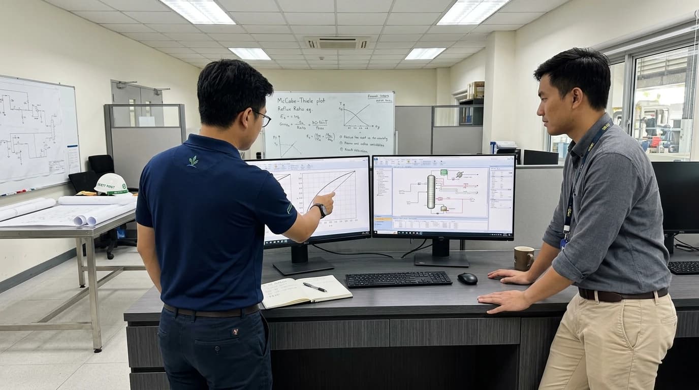
Determining whether to use NRTL or Peng-Robinson in a multi-component distillation simulation requires a clear evaluation of system composition, pressure, and chemical polarity. Choosing the wrong package causes massive deviations in VLE prediction, resulting in columns that either fail to converge or operate inefficiently in practice.
Polar vs. Non-Polar Behaviour
System polarity is the most significant factor when selecting a thermodynamic model. Non-polar mixtures, such as light alkanes, alkenes, and simple aromatics, exhibit highly predictable liquid phase behaviour. The Peng-Robinson equation of state excels at modelling these systems because the intermolecular forces are dominated by dispersion effects, which are well captured by the cubic attraction term.
However, when polar molecules such as water, alcohols, organic acids, or ketones are present, the liquid phase exhibits strong non-idealities due to hydrogen bonding and dipole-dipole interactions. Peng-Robinson cannot capture these localised molecular interactions, leading to gross errors. For example, when simulating an ethanol-water column, the Peng-Robinson model fails to accurately predict the binary azeotrope. This error can result in an underestimated reboiler duty, leading to insufficient separation and off-spec product. For these polar mixtures, the NRTL model is essential to resolve liquid-phase non-idealities.
Pressure Limits and Vapour Phase Ideality
The operating pressure of the column is another critical selection criterion. Because the NRTL model only calculates liquid activity coefficients, it treats the vapour phase using an auxiliary formulation, often assuming an ideal gas behaviour or using a simple virial equation. This approach is highly accurate at low to moderate pressures (typically under 10 bar) where vapour phase non-idealities are negligible.
At elevated pressures, such as those found in demethanisers or high-pressure refinery columns (often exceeding 20 bar), the vapour phase deviates significantly from ideal behaviour. The NRTL model's reliance on separate vapour formulations breaks down under these conditions. The Peng-Robinson model, by using a single cubic equation for both phases, models high-pressure systems and supercritical fluids with high precision.
Binary Interaction Parameters (BIPs)
Both models rely on parameters to adjust their predictions to match real-world experimental data. For NRTL, these parameters are the binary interaction parameters (τij and τji), which must be obtained from regression of experimental VLE data. If the simulator's databank lacks these parameters for a specific binary pair, the simulator often sets them to zero. This forces the NRTL model to calculate ideal liquid behaviour, completely defeating the purpose of using an activity model.
For Peng-Robinson, the binary interaction parameter (kij) adjusts the mixing rules for the attractive parameter. While kij parameters improve accuracy, Peng-Robinson is much less sensitive to missing parameters than NRTL when simulating simple hydrocarbon streams, allowing the column to converge with reasonable accuracy even when experimental data is sparse.
The following table summarises the comparative selection criteria for both models in industrial simulation:
| Operational Parameter | NRTL Model | Peng-Robinson (PR) EOS |
|---|---|---|
| Phase Modelling Basis | Liquid activity coefficient (γi), vapour via auxiliary EOS | Single cubic equation for both liquid and vapour phases |
| System Polarity | Highly polar, non-ideal, and associating mixtures | Non-polar to weakly polar systems |
| Operating Pressure | Low to moderate (typically under 10 to 15 bar) | Low to very high (including supercritical states) |
| Azeotrope Prediction | Highly accurate (requires regressed experimental BIPs) | Poor (cannot model structural hydrogen bonding) |
| Core Applications | Speciality chemicals, solvent recovery, bioethanol columns | Gas processing, oil refining, ethylene fractionation |
| Limitations | Unreliable at high pressures; dependent on BIP availability | Poor description of polar, highly non-ideal liquid phases |
To visualise the selection logic, process engineers can follow the systematic decision flow:
Real-World Scenario: Solvent Recovery Debottlenecking
To illustrate the financial and operational impact of model selection, consider a speciality chemical facility separating an isopropyl alcohol (IPA) and water mixture. This system forms a minimum-boiling azeotrope at approximately 80.3 °C with an IPA concentration of 68 mole percent.
If a design team attempts to model this separation using the Peng-Robinson equation of state, the simulation fails to capture the azeotropic point. It predicts a straightforward separation, leading the team to design a standard distillation column with too few stages and a low reflux ratio. In practice, this column would fail to produce high-purity IPA, requiring the plant to run at an excessively high reflux ratio to compensate. The resulting steam consumption in the reboiler would increase by over 30%, drastically raising utility costs and scope 1 carbon emissions.
By utilising the NRTL model, validated with accurate binary interaction parameters, the simulation accurately predicts the non-ideal VLE and the precise azeotropic composition. This allows the engineering team to design an extractive or azeotropic distillation column using an entrainer, or to couple the distillation with a membrane system. The reboiler heat duty is optimised, preventing energy waste and ensuring compliance with the Environmental Permitting Regulations.
Column Internals and Hydraulic Calculations
Thermodynamic accuracy also directly influences the physical sizing of column internals, whether utilising sieve trays, valve trays, or structured packing. Modern simulation platforms use the vapour and liquid traffic calculated from the mass balance to perform hydraulic rating calculations.
If the selected property package predicts inaccurate liquid densities or vapour pressures, the hydraulic model will yield flawed results for critical performance limits:
- Flooding: Occurs when the vapour flow rate is high enough to entrain liquid upwards to the tray above, causing a rapid increase in pressure drop and loss of separation efficiency.
- Weeping: Occurs when low vapour velocity allows liquid to rain down through the tray perforations instead of flowing across the active area, bypassing the mass transfer zone.
- Pressure Drop: High pressure drops in packed columns can damage heat-sensitive products by increasing the bottom temperature.
When simulation specialists use NRTL for low-pressure, highly non-ideal systems, the calculated liquid activity coefficients ensure accurate bubble point temperatures. This prevents overestimating the vapour density, leading to reliable tray flooding and pressure drop predictions. Underestimating these parameters via an incorrect Peng-Robinson simulation can cause premature column flooding in the physical plant, limiting throughput and disrupting debottlenecking schedules.
Overcoming Column Convergence Issues in Rigorous Simulation
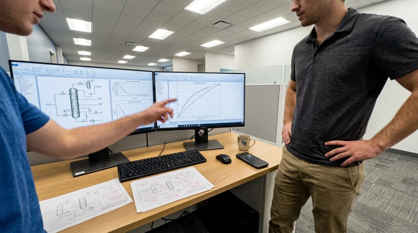
Once the thermodynamic package is selected, simulation specialists often encounter column convergence failures. Rigorous multi-component distillation columns represent some of the most numerically unstable unit operations in process modelling. Solving the underlying mathematical equations requires advanced numerical techniques and proper initialisation strategies.
The Inside-Out Method and Nested Solvers
Rigorous process simulation platforms (such as Aspen Plus's RadFrac or Aspen HYSYS) rely on advanced convergence algorithms like the "Inside-Out" method or nested two-tier mathematical solvers to handle highly non-linear mass and energy balances. First developed by Boston and Sullivan in the late 1970s, the Inside-Out method addresses the high computational cost of thermodynamic property evaluations.
The algorithm functions by dividing the problem into two distinct loops:
- The Inner Loop: This loop solves the material, equilibrium, stage sizing, and enthalpy (MESH) equations using simple, approximate thermodynamic models. Because these approximate models are mathematically simple, the inner loop converges rapidly.
- The Outer Loop: Once the inner loop converges, the outer loop evaluates the rigorous thermodynamic models (such as NRTL or Peng-Robinson) at the current stage temperatures and compositions. It uses these exact values to update the parameters of the approximate models in the inner loop.
This nested structure prevents the simulator from making expensive thermodynamic property calls during every single iteration, vastly improving convergence stability and speed.
Using Fenske-Underwood-Gilliland (FUG) Shortcut Design Equations
A frequent cause of solver divergence is a poor set of initial estimates for stage temperatures, liquid-vapour profiles, and product flows. When a simulation starts from ideal physical assumptions, the non-linearities of the columns can cause the solver to oscillate or hit boundary limits.
Resolving recycle loops and narrow boiling margins often requires establishing accurate initial estimates using traditional shortcut design equations (Fenske-Underwood-Gilliland).
- The Fenske Equation calculates the minimum number of theoretical stages (Nmin) at total reflux.
- The Underwood Equations determine the minimum reflux ratio (Rmin) based on feed thermal quality and relative volatilities.
- The Gilliland Correlation estimates the actual number of stages (N) for a specified operating reflux ratio (R).
By running a shortcut distillation block (such as DSTWU in Aspen Plus) prior to the rigorous column simulation, design engineers can calculate reliable estimates for stage requirements, feed location, and reflux ratios. Feeding these values as the initial profile into the rigorous column block ensures the solver starts close to the final solution, preventing mathematical divergence.
Troubleshooting Severe Convergence Failures
If a column fails to converge despite using a shortcut initialisation, simulation specialists must systematically diagnose the root cause.
- Check specifications: Verify that the specified product purities do not exceed thermodynamic limits. If the column is trying to separate a binary pair past its azeotropic limit without an entrainer, the solver will fail.
- Adjust solver parameters: In highly non-ideal liquid systems modelled with NRTL, standard acceleration methods can overcorrect, causing divergence. Switching the solver's convergence method from the default "Standard" to "Strongly Non-Ideal Liquid" or "Azeotropic" within the block options can improve stability.
- Apply damping: Damping parameters limit the step size taken by the Newton-Raphson solver during iterations, preventing the solver from oscillating between extreme values.
EnerTherm’s 11-Step Process Simulation Methodology
To bridge the gap between theoretical computer models and actual plant operations, industrial thermal engineering consultancies implement structured engineering methodologies. The proprietary 11-step engineering framework standardised by EnerTherm Engineering provides a unified, data-driven approach to resolving complex heat and mass balance (HMB) challenges.
From P&IDs and Historical Logs to the Single Source of Truth
The simulation process does not begin in a software environment. It begins with data acquisition.
- Project Scoping: Defining the physical boundaries of the study, environmental targets, and product specifications.
- P&ID Analysis: Examining piping and instrumentation diagrams to map the physical layout and column internals.
- Historical Log Gathering: Extracting real-world temperature, pressure, flow rate, and composition logs over extended operational periods.
- Data Reconciliation: Resolving inconsistencies in plant instruments to establish a mathematically closed mass balance.
Once the physical inputs are verified, process engineers proceed to thermodynamic package selection (such as NRTL or Peng-Robinson) and the construction of the steady-state simulation using industry-standard platforms.
Validating Steady-State and Dynamic Process Simulations
Developing a simulation is only valuable if the model replicates the actual behaviour of the operating asset under varying conditions.
- Flowsheet Construction: Laying out the column, reboiler, condenser, and auxiliary heat exchangers.
- Thermodynamic Model Alignment: Validating the VLE and enthalpy calculations against reliable experimental databases.
- Steady-State Solver Tuning: Adjusting efficiency parameters and tray heat losses to match historical operating profiles.
- Dynamic Transition: Transitioning the model into a dynamic simulation to test the column's response to process upsets, feed composition swings, and startup/shutdown procedures.
Energy Audits, Debottlenecking, and Decarbonisation Outcomes
The final steps of the methodology transform raw simulation data into physical plant improvements.
- Sankey Energy Mapping: Mapping all thermal inputs and outputs to identify where heat is lost or degraded.
- Debottlenecking Recommendations: Proposing concrete modifications, such as changing column internals, adjusting feed stage locations, or implementing heat integration.
- PFD Generation: Delivering a single-source-of-truth Process Flow Diagram (PFD) with embedded stream tables, mass and energy balances, and validated equipment sizing sheets.
Through this structured framework, chemical and petrochemical facilities achieve carbon mitigation, reduced utility costs, and rapid project payback periods. The resulting validated models serve as reliable guides for long-term capital investment and process optimisation.
This article reflects the independent analysis and editorial opinion of EnerTherm Engineering. Product names, trademarks, and brands mentioned belong to their respective owners. EnerTherm Engineering is not affiliated with, endorsed by, or a licensee of any third-party software or product mentioned unless explicitly stated.

Senior Process Engineer — EnerTherm Engineering
Masab Javed is a Senior Process Engineer at EnerTherm Engineering with extensive expertise in chemical process design, decarbonisation, and sustainable industrial solutions. He holds an MSc from TUM School of Management and a BEng in Chemical Engineering from NUST, with experience spanning ammonia production, CO2 capture, and semiconductor manufacturing optimisation.
